Lab3a

What is Xarray?

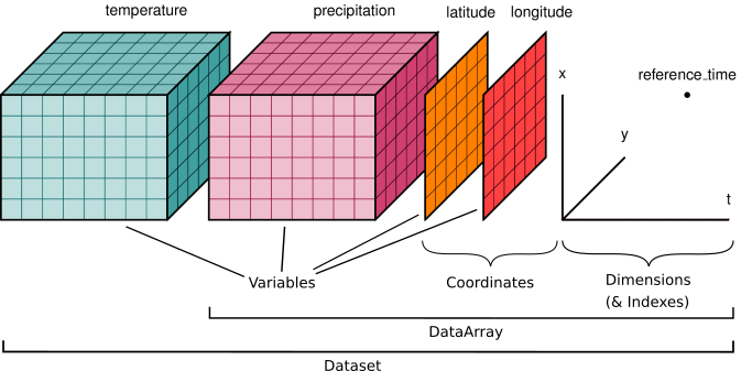
Xarray extends the capabilities of NumPy by providing a data structure for labeled, multi-dimensional arrays. The two main data structures in Xarray are:

• DataArray: A labeled, multi-dimensional array, which includes dimensions, coordinates, and attributes.

• Dataset: A collection of DataArray objects that share the same dimensions.

Xarray is particularly useful for working with datasets where dimensions have meaningful labels (e.g., time, latitude, longitude) and where metadata is important.

• rasterio: The main library for reading and writing raster data.

• rasterio.plot: A submodule of Rasterio for plotting raster data.

• numpy: A powerful library for array manipulations, which is very useful for raster data.

• matplotlib: A standard plotting library in Python for creating visualizations.

# %pip install xarray 

import xarray as xr
# This imports the pyplot module from matplotlib, a plotting library that provides functions for making a variety visualizations in Python.
import matplotlib.pyplot as plt

c:\Users\C00553090\AppData\Local\miniconda3\envs\hypercoast\lib\site-packages\pandas\core\computation\expressions.py:21: UserWarning: Pandas requires version '2.8.4' or newer of 'numexpr' (version '2.7.3' currently installed).
  from pandas.core.computation.check import NUMEXPR_INSTALLED

# Path to your Sentinel-2 NetCDF image
nc_file_path = './S2A_MSI_2016_09_20_16_44_50_T15RYN_L2W_subset.nc'

# Open the NetCDF file，this line uses xarray's open_dataset function to load the NetCDF file specified by nc_file_path into the variable ds. 
# The ds variable now contains an xarray.Dataset object, which is a multi-dimensional, in-memory array database. 
# Rhis dataset likely contains various data variables such as spectral bands and other metadata.

ds = xr.open_dataset(nc_file_path)

# Check available variables (bands) in the dataset
print("Variables in the dataset:", ds.data_vars)

Variables in the dataset: Data variables:
    Rrs_443             (y, x) float32 175MB ...
    Rrs_492             (y, x) float32 175MB ...
    Rrs_560             (y, x) float32 175MB ...
    Rrs_665             (y, x) float32 175MB ...
    Rrs_704             (y, x) float32 175MB ...
    Rrs_740             (y, x) float32 175MB ...
    Rrs_783             (y, x) float32 175MB ...
    Rrs_833             (y, x) float32 175MB ...
    Rrs_865             (y, x) float32 175MB ...
    Rrs_1614            (y, x) float32 175MB ...
    Rrs_2202            (y, x) float32 175MB ...
    l2_flags            (y, x) int32 175MB ...
    chl_oc3             (y, x) float32 175MB ...
    chl_re_mishra       (y, x) float32 175MB ...
    SPM_Nechad2016_665  (y, x) float32 175MB ...

# Extract the necessary variables (TSS and Rrs_665)

red = ds['Rrs_665'].values
green = ds['Rrs_560'].values
NIR1 = ds['Rrs_704'].values
NIR2 = ds['Rrs_740'].values
NIR3 = ds['Rrs_833'].values
# Make sure lon and lat are 1D arrays
lon = ds['lon'].values
lat = ds['lat'].values

# Calculate TSS using the formula (Miller & McKee, 2004)
# https://www.sciencedirect.com/science/article/pii/S0034425704002317
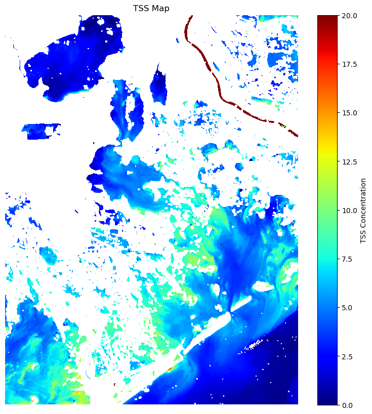
TSS_Miller = 1140.25 * red - 1.91

# Optional: Display the TSS map
plt.figure(figsize=(10, 10))
plt.imshow(TSS_Miller, cmap='jet', vmin=0, vmax=20)
plt.colorbar(label='TSS Concentration')
plt.title('TSS Map')
plt.axis('off')
plt.show()

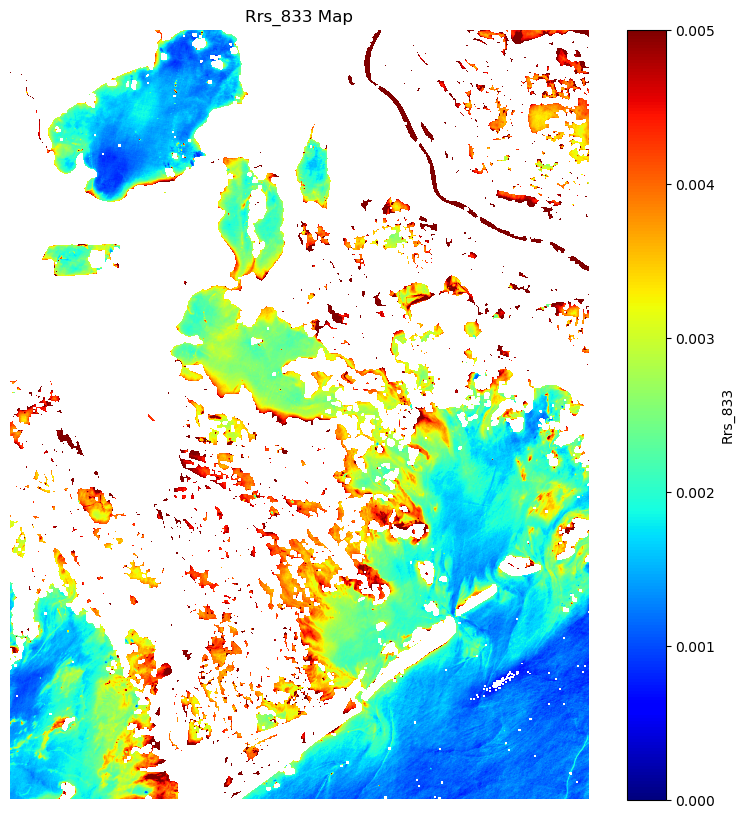
# Optional: Display the Rrs_665 map
plt.figure(figsize=(10, 10))
plt.imshow(NIR3, cmap='jet', vmin=0, vmax=0.005)  # You can choose a different colormap
plt.colorbar(label='Rrs_833')
plt.title('Rrs_833 Map')
plt.axis('off')
plt.show()

Reading Raster Data

To read raster data, you can use the rasterio.open() function. This function creates a connection to the file without loading the entire dataset into memory. This is particularly useful for large datasets like satellite imagery or high-resolution DEMs, as they might be too big to fit into memory at once.

import rasterio
import rasterio.plot
from rasterio.transform import from_origin

# Create transform using top-left corner (lon.min(), lat.max()) and pixel size

# The from_origin(lon.min(), lat.max(), pixel_size_x, pixel_size_y) function creates a transformation matrix that starts at the top-left corner 
# of the image (where lon.min() and lat.max() are) and applies the pixel sizes to convert the image into a geospatial format that software 
# like QGIS, ArcGIS, or any other GIS tool can interpret.
# The transform provides a way to map between pixel coordinates (like row/column in an array) and real-world coordinates (latitude/longitude). 
# Without this, the image would not be tied to any specific place on Earth.

pixel_size_x = (lon.max() - lon.min()) / red.shape[1]
pixel_size_y = (lat.max() - lat.min()) / red.shape[0]
transform = from_origin(lon.min(), lat.max(), pixel_size_x, pixel_size_y)

# Define the output GeoTIFF filename
output_tif = 'TSS_and_Rrs_12082015_lab1.tif'


# Save both the TSS concentration and Rrs as bands in the GeoTIFF
# The rasterio.open function is used here with the 'w' option to open a file for writing:
with rasterio.open(
    output_tif,
    'w',
    driver='GTiff',
    height=TSS_Miller.shape[0],
    width=TSS_Miller.shape[1],
    count=6,  # Two bands: one for TSS and one for Rrs_665
    dtype=TSS_Miller.dtype,  # Assuming both have the same data type
    crs='EPSG:4326',
    transform=transform,
) as dst:
    # Writing Data to the GeoTIFF within the opened file context (dst), multiple data arrays are written to different bands of the GeoTIFF:
    dst.write(TSS_Miller, 1)  # Write TSS concentration to the first band
    dst.write(red, 2)  # Write Rrs_665 to the second band
    dst.write(green, 3) # 
    dst.write(NIR1, 4)  # 
    dst.write(NIR2, 5)  # 
    dst.write(NIR3, 6)  #

print(f'Saved {output_tif}')

Saved TSS_and_Rrs_12082015_lab1.tif

raster_path = './TSS_and_Rrs_12082015_lab.tif'
src = rasterio.open(raster_path)
print(src)

<open DatasetReader name='./TSS_and_Rrs_12082015_lab.tif' mode='r'>

File Name: The name attribute gives you the file path or URL of the opened raster.

src.name

File Mode: The mode attribute shows how the file was opened. For example, a raster can be opened in read-only (‘r’) or write (‘w’) mode.

src.mode

Raster Metadata: The meta attribute provides key information about the raster, such as its width, height, CRS, number of bands, and data type.

src.meta

The CRS describes how the 2D pixel values relate to real-world geographic coordinates (latitude and longitude or projected coordinates). Knowing the CRS is essential for interpreting the data in a meaningful way. To retrieve the CRS:

src.crs